Define complexity of the algorithm. Explain asymptotic notations.

Define complexity of the algorithm. Explain asymptotic notations.  

Answer :when we want an estimate of the running time or other resource requirements of an algorithm. the analysis and keeps us thinking about the most

important aspect: the growth rate. it is called asymptotic algorithm analysis To be precise, asymptotic analysis refers to the study of an algorithm as the input

size “gets big” or reaches a limit (in the calculus sense). However, it has proved to be useful to ignore all constant factors it  asymptotic analysis is used for most algorithm comparisons

Asymptotic is a form of “back of the envelope” estimation for algorithm resource consumption. It provides a simplified model of the

running time or other resource needs of an algorithm. This simplification usually helps you understand the behavior of your algorithms. Just be aware of the limitations to asymptotic analysis in the rare situation where the constant is importent

The following 3 asymptotic notations are mostly used to represent time complexity of algorithms.

1) Θ Notation: big-Oh and Ω give us ways to describe the upper bound for an algorithm (if we can find an  equation for the maximum cost of a particular class of inputs of size n ) and the lower bound for an algorithm (if we can find an equation for the minimum cost or a particular class of inputs of size n ). When the upper and lower bounds are the same within a constant factor, we indicate this by using Θ (big-Theta) notation.   algorithm is said to be Θ(h(n))if it is in O(h(n)) and it is in Ω(h(n)) . Note that we drop the word “in” for Θ notation, because there is a strict equality for two equations the same Θ . In other words, if f (n)is Θ( g ( n)), then g ( n ) is Θ(f(n)) .Because the sequential search algorithm is both in O( n) and inΩ( n)in the average case, we say it is Θ(n)in the average case. Given an algebraic equation describing the time requirement for an algorithm, the upper and lower bounds always meet. That is because in some sense we have a perfect analysis for the algorithm, embodied by the running-time equation

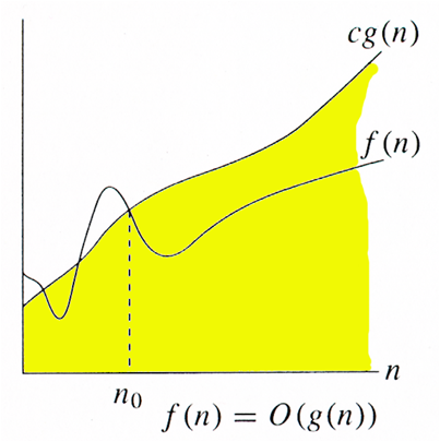
The Big O notation defines an upper bound for the growth of the algorithm’s running time. It indicates upper or highest growth rate that the algorithm can have. To make any statement about the upper bound of an algorithm, we must be making it about some class of inputs of size n . We measure this upper bound nearly always on the best-case, average-case, or worst-case inputs. Thus, we cannot say, “this algorithm has an upper bound to its growth rate of n2.” We must say something like, “this algorithm has an upper bound to its growth rate of n2 in the average case .” Because the phrase “has an upper bound to its growth rate off (n)” is long and often used when discussing algorithms, we adopt a special notation, called big-Oh notation. If the upper bound for an algorithm’s growth rate (for, say, the worst case) is f(n), then we would write that this algorithm is “in the set O(f(n)) in the worst case” (or just “in O(f(n)) in the worst case”)
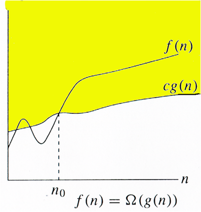
3) Ω Notation: Ω Notation< can be useful when we have lower bound on time complexity of an algorithm. The lower bound for an algorithm (or a problem, as explained later) is denoted

by the symbol Ω , pronounced “big-Omega” or just “Omega.” The following definition for Ω is symmetric with the definition of big-Oh. For T (n)a non-negatively valued function, T(n) is in set Ω(g(n))if there exist two positive constants c and n 0such that T (n) ≥cg (n)for all n > n 0. 1

What is Queue? Describe the two ways of implementing the Queue.

Answer: Queue is a list-like structure that provides restricted access to its elements. Queue elements can only be inserted at the back (this is called an enqueue operation) and removed from the front (called a dequeue operation) .

Example: Queues operate like standing in line at a movie theater ticket counter. If nobody cheats, then newcomers go to the back of the line. The person at the front of the line is the next to be served. Thus, queues release their elements in order of arrival

Two way of implementing the Queue:

1. The array-based Queue

2. The linked queue

The Array based :

Assume that there are n elements in the queue. By analogy to the array-based list implementation, we could require that all elements of the queue be stored in the first n positions of the array. If we choose the rear element of the queue to be in position 0, then dequeue operations require only Θ(1) time because the front element of the queue (the one being removed) is the last element in the array.

20 front

5

12

17 rear

 (a)

12 front

17

3

30

4 rear

(b)

After repeated use, elements in the array-based queue will drift to the back of the array. (a) The queue after the initial four numbers 20, 5, 12, and 17 have been inserted. (b) The queue after elements 20 and 5 are deleted, following which 3, 30, and 4 are inserted.

we chose the rear element of the queue to be in position n − 1 , then an enqueue operation is equivalent to an append operation on a list. This requires only Θ(1) time. But now, a dequeue operation requires Θ( n) time, because all of the elements must be shifted down by one position to retain the property that the remaining n−1 queue elements reside in the first n −1 positions of the array

Link queue :

The linked queue implementation is a straight forward adaptation of the linked list. Methods front and rear are pointers to the front and rear queue elements, respectively. We will use a header link node, which allows for a simpler implementation of the enqueue operation by avoiding any special cases when the queue is empty. On initialization, the front and rear pointers will point to the header node, and front will always point to the header node while rear points to the true last link node in the queue  enqueue places the new element in a link node at the end of the linked list (the node that rear points to) and then advances rear to point to the new link node. Method dequeue grabs the first element of the list removes it .

Program Example :

class LQueue<E> implements Queue<E> {

private Link<E> front; // Pointer to front queue node

private Link<E> rear; // Pointer to rear queuenode

int size; // Number of elements in queue

// Constructors

public LQueue() { init(); }

public LQueue(int size) { init(); } // Ignore size

private void init() { // Initialize queue

front = rear = new Link<E>(null);

size = 0;

}

public void clear() { init(); } // Reinitialize queue

public void enqueue(E it) { // Put element on rear

rear.setNext(new Link<E>(it, null));

rear = rear.next();

size++;

}

public E dequeue() { // remove element from front

assert size != 0 : "Queue is empty";

E it = front.next().element(); // Store dequeued value

front.setNext(front.next().next()); // Advance front

if (front.next() == null) rear = front; // Last Object

size--;

return it; // Return Object

}

public E frontValue() { // Get front element

assert size != 0 : "Queue is empty";

return front.next().element();

}

public int length() { return size; }

Question 3. Write a note on the advantages and disadvantages of Linear and linked representation of tree

Answer: A linear  is an index file organized as a sequence of key/pointer pairs where the keys are in sorted order and the pointers either (1) point to the position of the complete record on disk, (2) point to the position of the primary key in the primary index

Advantages of Linear :

It provides convenient access to variable-length database records, because each entry in the index file contains a fixed-length key field and a fixed-length pointer o the beginning of a (variable-length) record as shown in Figure 10.1. A linear index also allows for efficient search and random access to database records, because it is amenable to binary search. if the database contains enough records, the linear index might be too large to store in main memory. This makes binary search of the index more expensive because many disk accesses would typically be required by the search process. One solution to this problem is to store a second-level linear index in main memory that indicates which disk block in the index file stores a desired key.

Disadvantages :

A drawback to this approach is that the array must be of fixed size, which imposes an upper limit on the number of primary keys that might be associated with a  particular secondary key. Furthermore, those secondary keys with fewer records than the width of the array will waste the remainder of their row. A better approach is to have a one-dimensional array of secondary key values, where each secondary key is associated with a linked list. This works well if the index is stored in main memory, but not so well when it is stored on disk because the linked list for a given key might be scattered across several disk blocks.

linked representation of tree:

B-trees are always height balanced, with all leaf nodes at the same level.

2.Update and search operations affect only a few disk blocks. The fewer the number of disk blocks affected, the less disk I/O is required.

3.B-trees keep related records (that is, records with similar key values) on the same disk block, which helps to minimize disk I/O on searches due to locality of reference

Question 2 . Discuss the following storage allocation: 

(a) Fixed block (b) Variable block  

Answer:

(a) Fixed block

Fixed block allocation, is also called memory pool allocation, uses of a free list of fixed  block of memory is often all of the same size. This works well for simple embedded systems where it's no large objects need to be allocated, but it suffers from fragmentation, especially with long memory addresses.

Example of

Fixed block allocation. operating system divides the main memory into equal number of fixed sized partitions, operating system occupies some fixed portion and remaining portion of main memory is available for user processes.

Any process whose size is less than or equal to the partition size can be loaded into any available partition.

like if we define array size of 10 that means array can take only 10 element . so advantages

of this declaration if we are working on small project or always fix size type of allocation that time we use this fix size block allocation.  

(b) Variable block  

This section with the general case where blocks of any size might be requested and released in any order. This is known as Variable block storage allocation Variable block storage allocation, we view memory as a single array broken into a series of variable-size blocks, where some of the blocks are free and some are reserved or already allocated. The free blocks are linked together to form a free-list used for servicing future memory request Memory managers can suffer from two types of fragmentation. External fragmentation occurs when a series of memory requests result in lots of small free blocks, no one of which is useful for servicing typical requests. in Variable block storage allocation has Internal fragmentation occurs when more than m words are allocated to a request for m words, wasting free storage. This is equivalent to the internal fragmentation that occurs when files are allocated in multiples of the cluster size.

Question 3 :Define sorting. With suitable example describe merge sort.

Answer: Sorting is a technique to arranging data in particular order.  Sorting is also one of the most frequently performed computing tasks . we might use sorting as an intrinsic part of an algorithm to solve some other problem, such as when computing the minimum-cost spanning tree The collection of sorting algorithms presented that divide and-conquer is a powerful approach to solving a problem, and that there are multiple ways to do the dividing. Mergesort divides a list in half.

Merge sort:A natural approach to problem solving is divide and conquer. In terms of sorting, we might consider breaking the list to be sorted into pieces, process the pieces, and then put them back together somehow. A simple way to do this would be to split the list in half, sort the halves, and then merge the sorted halves together. his is the idea behind Mergesort . Mergesort is one of the simplest sorting algorithms conceptually, and has good performance both in the asymptotic sense and in empirical running time

pseudocode for Merge sort

List mergesort(List inlist)

{

if (inlist.length() <= 1) return inlist;;

List l1 = half of the items from inlist;

List l2 = other half of the items from inlist;

return merge(mergesort(l1), mergesort(l2));

}

Merging two sorted sublists is quite simple. Function merge examines the first element of each sublist and picks the smaller value as the smallest element overall. This smaller value is removed from its sublist and placed into the output list. Merging continues in this way, comparing the front elements of the sublists and continually appending the smaller to the output list until no more input elements remain